Statistics Module - Using NumPy, SciPy, Matplotlib to represent data

Throughout this series, I have mentioned the concepts of data and information several times, as well as how data is processed into information. Information that we can use within our programs or make meaningful information for decision-making processes.

This module, in particular, focuses on how we can use the statistics module/library within Python to extrapolate information from numerical data. This is especially useful for statisticians who spend most of their time working with numerical data and mathematical functions.

These modules focus on performing complex operations on numerical inputs, helping to retrieve detailed information such as graphs, coordinates, arrays, etc. The original course contents make mention of most developers coming across the need to use this module, as we all encounter using statistics at some point of our programming journey.

This module is very theory heavy, explaining and elaborating on a large amount of functions available that we can use for statistics. There are also different modules that we can install/import into our Python program, which give us different levels of insights depending on our need.

As an entry level developer using Python, I’ll make an attempt to go through the course contents and provide as much information as I can about what I learn. On my first iteration of this module, I missed out on using some of the functions like matplotlib, where I am able to display a graph in our terminal using numerical data.

This should enable me to gain the correct depth of knowledge I need to then use or keep in mind when it comes to coding with Python.

Statistics Modules

Python comes with a pre-built statistics module that lets us calculate complex mathematical operations like standard deviation, variance, mean, mode, etc. To use the module, you would just go ahead and import the module and use it as usual.

Python also has several packages that we can install for different levels or layers of depth when it comes to stats.

namely, we have:

• MatPlotLib
• NumPy (Numerical Python)
• Scipy
• Pandas

For more advanced methods, we have:

• Minitab
• SAS
• Matlab

Most of the course content for this topic only goes over using the NumPy functions and methods available. It would be a good idea to go ahead and use the rest of the modules listed, but for now, I’ll keep it as relevant as I can to the course itself.

One of the requirements made in the course is to download and install Jupyter Notebook which is used as a development environment like VS Code but for working with statistics or even machine learning libraries. A benefit to using Jupyter Notebook is being able to do incremental experimentation and use more visual feedback than in VS Code, as this is more project based and structured.

pip install jupyterlab

Once it’s installed, you can then load the application by running the following line of code in the terminal:

jupyter lab

After a few moments, you should be able to have the Jupyter Notebook or Lab opened on a browser:

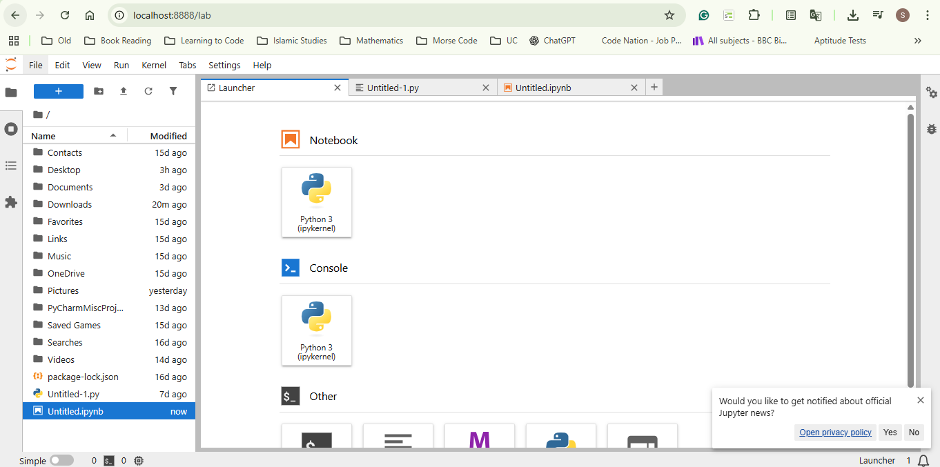
Now we would click on the option to create a new Python file in Jupyter that is located directly under Notebook. This then would load something different to what a typical Python file would look like. You can view the differences between the two file types when you open one that was created with the Notebook and the other as a regular Python file.

With all that done and out of the way, we can now focus on using some of the installed packages.

Using NumPy (Numerical Python or Number Python)

First, we have to install the NumPy package on to our development environment, use a virtual environment if required. Inside Jupyter Notebook, open the terminal, which should be located at the bottom and run the following code:

pip install numpy

Now that we have NumPy installed, we can have our functions embedded inside Jupyter Lab and go ahead and use them. If, for whatever reason, this hasn’t worked, just re-open Jupyter Lab and start again.

NumPy Arrays

We’ve already had a whole topic on arrays and explaining their uses, but I want to include some nuances here that will help later when it comes to dealing with arrays, especially in NumPy.

To use NumPy, we would begin by importing the module into our file.

import numpy as np

Tip: This is creating an abbreviation for our module to be used throughout our code. Instead of having to refer to the module using NumPy. we can now use np. which will work the same - again, try refrain from using any of the reserved words.

We can go ahead and create an array of numbers as we usually would using Python:

num_array = [1,2,3,4,5]

We’ve already practised using functions with normal lists, so let’s change this list to being a NumPy list/array.

NumPy_array = np.array(num_array)
print(NumPy_array)
#Output:
# [1,2,3,4,5]

The new list will be classified as a NumPy array or data type.

print(type(NumPy_array))
#Output:
# NumPy.ndarray

Using this method, we can take the contents of a list and change it to a different data type, like the following:

NumPy_array1 = np.array(num_array, dtype = float) # Change each digit to a decimal figure
# We can also insert the list manually:
NumPy_array2 = np.array([1,-1,0,0,1], dtype = bool) # Change each digit to a Boolean

print(NumPy_array1) # [1.,2.,3.,4.,5.]
print(NumPy_array2) # [True, True, False, False, True]

We still have access to similar operations like len(), which brings us the total number of items in a list, just using a different syntax:

lst = [1,2,3,4,5]
np_lst = np.array(lst)

print(np_lst.size)
# 5

Multi-Dimensional Arrays

There is a concept known as multi-dimensional arrays, which I briefly explained in an earlier post. To shed some more light on this topic, which I believe is more accurate, this is how to view them.

# can be a normal list, tuple, etc
[1,2,3,4,5] # 1D array (Vector)
[[1,2],[3,4]] # 2D array (Matrix)

[# list a
    [ #list b
        [1,2],[1,2] # list c & d
        ],
    [
        [3,4], [3,4]
        ]
    ] # 3D array (Tensor)

With NumPy, we can also obtain the shape of a multi-dimensional array (number of columns and rows), which could be useful information.

NumPy_array = np.array(
    [
    (1,2,3),
    (4,5,6),
    (7,8,9)
    ]
    )
print('Shape: ', NumPy_array.shape)
# (3, 3) (3 columns and 3 rows)

You can access the items within a multi-dimensional array using the same method as indexing in a list.

NumPy_array = np.array([[1,2],[3,4],[5,6]]) # Matrix array

first_row = NumPy_array[0]
print(first_row) # [1,2]

# We can instead get the first item of each list to form our column:
column1 = NumPy_array[:,0]
# This is using the slicing method.
# The syntax for this is: [rows: , columns] otherwise, it will treat as normal list slicing method
# give me column index 0 for every row
print(column1) # [1,3,5]

Slicing NumPy Arrays

We can perform the same slicing operations on NumPy arrays; we just have to keep the syntax in mind.

[rows, columns]

array = np.array([[1,2,3],[4,5,6],[7,8,9]])

first_two_columns = array[0:2, 0:2]
print(first_two_columns)

# [1,2]
# [4,5]

reverse = array[::-1,::-1] # reverse the main list and also the list inside (2D)
print(reverse)
[[9 8 7]
 [6 5 4]
 [3 2 1]]

Rearranging NumPy Arrays

Interestingly, we can reshape the arrays that we retrieve by even flattening them or reshaping the contents inside to form a new list.

first_shape = np.array([(1,2,3), (4,5,6)])
reshaped = first_shape.reshape(3,2)
flattened = reshaped.flatten()
print(reshaped)
#   [[1 2]
#    [3 4]
#    [5 6]]
print(flattened)
# [1 2 3 4 5 6]

Hint: NumPy has its own random module which can be used for random number generations or functions.

Data Types - Re-explained

A while ago, I made a post on data types available within Python and that there were 2 primary types of data we can find in Python

1. Primitive (built-in or core data types like Float, String, Boolean)
2. Abstract/Complex (data types derived from complex operations or functions)

Here, we can see this in action.

When we use NumPy to take an existing set of data and translate that to it’s own set of digits or array, we do also convert that list to a NumPy specific data type. Whether that’s a float, integer, boolean etc. it becomes a form of abstract data type.

The reason why I used the word form is that an abstract data type is described as being a rule and not a representation. An abstract data type would be the following:

ADT	What It Represents
Stack	Last-in, first-out collection
Queue	First-in, first-out collection
Deque	Add/remove from both ends
Set	Unique elements
Map / Dictionary	Key–value associations
List (logical)	Ordered sequence

This did help me understand this a little more.

To deepen my explanation, think of NumPy using it’s own set of data types for each digit or representation of data. For example, where usually in Python print(type(5)) would give us int for a NumPy number, it would give us int64.

These are the data types in NumPy:

Python type	NumPy equivalent
int	np.int32, np.int64
float	np.float32, np.float64
bool	np.bool_
complex	np.complex64, np.complex128

At this point, I won’t be able to explain why they differ or what they do. After speaking with ChatGPT, which gave me both those lists, I can say that in both scenarios we can think of the digits as being objects as we learnt of in classes and objects.

The figures provided to us by NumPy seem to be more restrictive, whereas without NumPy, they are less restrictive.

Earlier, I made an illustration on how to change the data type of a NumPy list, and now let me provide another example, which is from the original course:

lsta = [1,2,3,4,5]
NumPy_list = np.array(lsta)

print(NumPy_list.astype('int').astype('str')) # ['1', '2', '3', '4', '5']

This will change each int64 to a string type.

Mathematical Operations With NumPy

Surprisingly, NumPy’s operations for mathematical functions seem to be easier to use.

lsta = [1,2,3,4,5]
NumPy_list = np.array(lsta)

add_ten = NumPy_list + 10 # Adds to every item in the list
print(add_ten) # [11, 12, 13, 14, 15]

minus_ten = NumPy_list - 10
print(minus_ten) # [-9, -8, -7, -6, -5]

multiply_ten = NumPy_list * 10
print(multiply_ten) # [10, 20, 30, 40, 50]

# We can do the same for division (/), floor division(//), exponent (**), and modulus (%).

We didn’t have to use a loop function for it to iterate through each item in the loop with NumPy, and it’s made the whole process simpler. This is what we would call refactored code - easier, efficient, and effective code used to obtain the same result.

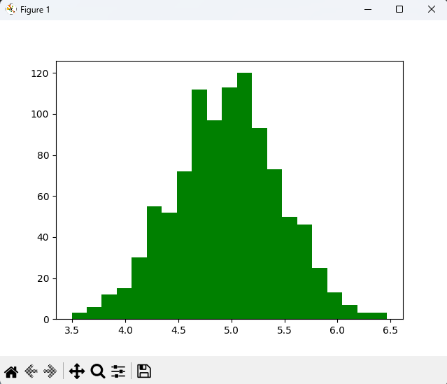
Using Graphs With NumPy

Something that I find quite useful within this topic is the ability to generate a graph using matplotlib. This function helps data scientists or those involved with data extraction to curate meaningful information from a dataset.

import numpy as np
import matplotlib.pyplot as plt

numpy_array = np.array([[1,2,3],[4,5,6],[7,8,9]])

np_normal_dis = np.random.normal(5, 0.5, 1000)
print(np_normal_dis)

plt.hist(np_normal_dis, color="green", bins=21)
plt.show() # Opens a window with a graph

Functions in NumPy

I’ve had a brief read through again of the course materials, and though I have a slighter insight into using NumPy arrays and their functions. I don’t want to have them all listed and explained in my blog post.

This would make it far too long a post. What I would rather do is collate the information in a manner that is better understood than experimented with. This will give me the knowledge of knowing the tools available and only practice with them when the need arises, as this is a very distinct topic when it comes to using them.

NumPy Core & Array Creation

Function / Attribute	What it Does	Syntax	Example	Output
np.array()	Creates a NumPy array	np.array(iterable, dtype=None)	np.array([1,2,3])	[1 2 3]
dtype	Sets data type	np.array([1,2], dtype=float)	[1., 2.]	float array
np.zeros()	Creates array of zeros	np.zeros((r,c))	np.zeros((2,2))	[[0 0],[0 0]]
np.ones()	Creates array of ones	np.ones((r,c))	np.ones((2,2))	[[1 1],[1 1]]
np.matrix()	Creates matrix object	np.matrix(arr)	np.matrix([[1,2],[3,4]])	matrix

Array Properties

Property	Purpose	Syntax	Example	Output
.shape	Rows & columns	arr.shape	(3,3)	tuple
.size	Total elements	arr.size	9	int
.dtype	Data type	arr.dtype	int64	type
.itemsize	Bytes per element	arr.itemsize	8	bytes

Indexing & Slicing

Operation	Meaning	Syntax	Example	Output
Row access	Get a row	arr[0]	[1 2 3]	row
Column access	Get column	arr[:,0]	[1 4 7]	column
Slice	Sub-array	arr[0:2,0:2]	[[1 2],[4 5]]	array
Reverse	Reverse rows	arr[::-1]	reversed	array
Reverse both	Flip rows & cols	arr[::-1,::-1]	reversed	array

Type Conversion

Conversion	Syntax	Example	Output
Int → Float	astype(float)	[1,2] → [1.,2.]	float
Float → Int	astype(int)	[1.5] → [1]	int
Int → Bool	dtype=bool	[-1,0,2]	[T,F,T]
Any → Str	astype(str)	[1,2]	['1','2']

Mathematical Operations (Vectorised)

Operation	Syntax	Example	Output
Add	arr + 10	[1,2]+10	[11,12]
Subtract	arr - 10	[1,2]-10	[-9,-8]
Multiply	arr * 2	[1,2]*2	[2,4]
Divide	arr / 2	[2,4]/2	[1.,2.]
Modulus	arr % 3	[4]%3	[1]
Power	arr ** 2	[2]**2	[4]

Reshaping & Stacking

Function	Purpose	Example	Output
reshape()	Change shape	(2,3)→(3,2)	reshaped
flatten()	1D array	[[1,2],[3,4]]	[1 2 3 4]
np.hstack()	Horizontal join	[1,2],[3,4]	[1 2 3 4]
np.vstack()	Vertical join	[1,2],[3,4]	[[1 2],[3 4]]

Sequence Generation

Function	Purpose	Example	Output
np.arange()	Range values	np.arange(1,10,2)	[1 3 5 7 9]
np.linspace()	Even spacing	linspace(1,5,5)	floats
np.logspace()	Log scale	logspace(2,4,4)	powers
np.tile()	Repeat array	tile([1,2],2)	[1 2 1 2]
np.repeat()	Repeat elements	repeat([1,2],2)	[1 1 2 2]

Random Number Generation (np.random)

Function	Purpose	Example	Output
random()	Float [0,1)	np.random.random()	0.53
rand()	Shape floats	np.random.rand(2,2)	matrix
randn()	Normal dist	np.random.randn(2,2)	normal
randint()	Random ints	randint(0,10,(2,2))	ints
choice()	Random pick	choice(['a','b'],3)	values
normal()	Gaussian	normal(mu,sigma,n)	array

Statistical Functions

Function	Purpose	Example	Output
np.min()	Minimum	np.min(arr)	value
np.max()	Maximum	np.max(arr)	value
np.mean()	Average	np.mean(arr)	float
np.median()	Middle	np.median(arr)	value
np.std()	Std deviation	np.std(arr)	float
np.var()	Variance	np.var(arr)	float
np.amin(axis)	Min per axis	axis=0	array
np.amax(axis)	Max per axis	axis=1	array

Linear Algebra

Function	Purpose	Example	Output
np.dot()	Dot product	[1,2]·[3,4]	11
np.matmul()	Matrix multiply	A@B	matrix
np.linalg.det()	Determinant	det([[5,6],[7,8]])	-2

Summary

I didn’t write about all the individual functions available inside the NumPy module. It’s important that I go over and use the functions instead of writing all about them as per the course requirements. I wanted this post to be as concise as possible and to refrain from completely replicating the initial set of instructions inside the course’s content for this topic.

With that being said, I will spend more time using this information, and if there are any updates, I will try and include them here as I go on to learn to using NumPy.